


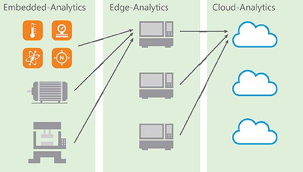
Figure 1: With each step from right to left, less computing capacity and storage space are available, i.e. big data must become smart data and instead of extensive algorithms, lean, self-learning algorithms are required. (Image source: Knowtion)
Rutroniker: Mr. Mangler, you and your team have developed algorithms that require neither a cloud nor a high-performance PC but run on a microcontroller. Why?
Andreas Mangler: We see a clear move in many industrial applications away from having data analyzed and evaluated externally by a service provider (cloud analytics) or a decentralized industrial PC (edge analytics) and toward having everything implemented in an separate protected environment as an embedded MCU-based system (embedded analytics). And all of this ideally with appropriate hardware encryption. IP protection and real-time capability of the system are at the center of decisions in favor of embedded analytics, in particular the protection of the raw data, the algorithms used, and their sequential sequencing in order to finally obtain the desired information from big data. And yet, embedded analytics systems are usually based on mathematical models, patterns, and functions with which a target/actual comparison is carried out using the data already learned and the measured data.
Many tasks therefore not only involve pattern matching, which is not necessarily only available in the image processing of graphic data, but the processing of a large amount of sensor data with varying physical measured variables, which are typically processed time synchronously; the keyword here is sensor fusion.
An embedded analytics solution is indispensable, especially in safety-relevant systems or where functional safety is required in real time and quasi ad-hoc decisions have to be made in the microsecond or nanosecond range.
One measure, for example, is the use of stochastic filters, which can be well supported by the MCU’s memory organization. Another option is to use IIR filters instead of block-oriented FIR filtering as the digital filters, taking into account the different group delay and transient response of the filter topologies.
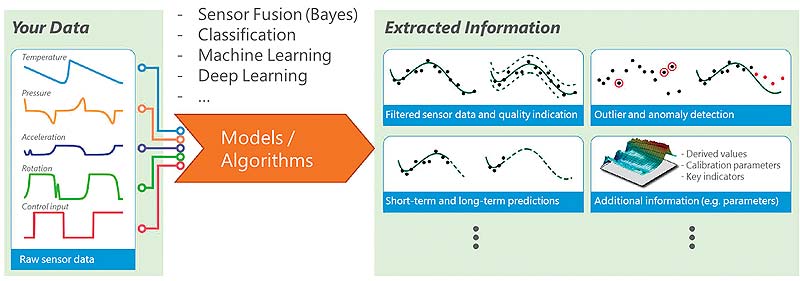
Figure 2: Principle of sensor fusion and data extraction. (Image source: Knowtion)
This actually sounds quite simple, but most probably it isn’t. In a real-life scenario, how can such large amounts of data and algorithms be processed in a small microcontroller?
The problem of sensor fusion is well described by the buzzword VUCA, i.e. Volatility, Uncertainty, Complexity, and Ambiguity. Volatility arises because the system is constantly changing in terms of its data, dynamics, speed, and limits. Uncertainties exist, e.g., due to noise and unforeseeable events. In addition, the systems are typically complex and there are ambiguities, as some states may have different causes. The aim is to assess this “hidden” information in order to better describe the system. Data can already be reduced through the previous rough estimation of the actual state.
For example, a heating control system for a gas heater that has to carry out a CO2 analysis could determine the exact outside temperature in parallel. This way, when used in Norway, the heater can certainly take a winter temperature of -30°C into account when calculating the measured value. In southern Spain, this temperature is extremely unlikely, or downright unrealistic, in the winter. Consequently, the GPS location sensor or logistics data of the heater supplier determines the amount of data to be evaluated.
The formula is: Data reduction plus lean algorithms that are combined correctly. This requires four steps: Firstly, sensor deployment planning, i.e. how many sensors of which sensor type are required where? The second step concerns data selection, i.e. the question: Which data is actually required to detect anomalies? This is how “big data” becomes “smart data”. Above all, the trick here is to select as much data as necessary and as little as possible, while still managing to pick the right data. In the third step, the algorithms for pre-filtering need to be selected. The parameters required for analysis are then extracted in the fourth step. All the steps have to be precisely adapted to the system and the actual problem. Furthermore, the basic problem of synchronous data processing has to be considered for sensor fusion.
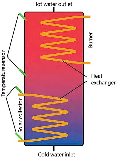
Figure 3: Schematic design of a hot water tank with a PV system and several temperature sensors. (Image source: Knowtion)
How can this be implemented in the MCU?
The physical system and the possible states in reality are considered and described for this purpose. This then leads to an assessment of the state. These types of model can be defined in advance in the laboratory and stored in the microcontroller’s look-up table. The sensor data can then be compared with the model and outliers can quickly be identified as an anomaly. This means fewer measuring points are required, which in turn helps to save storage space.
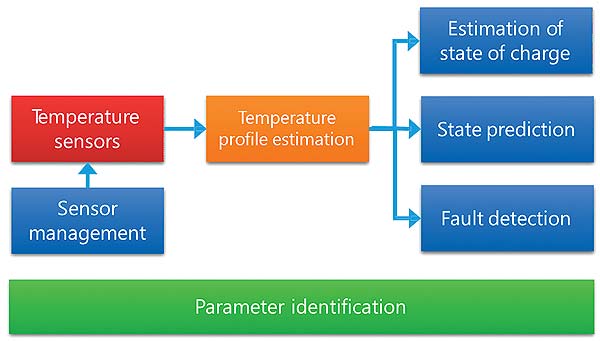
Figure 4: Principle of parameter identification and anomaly detection. (Image source: Knowtion)
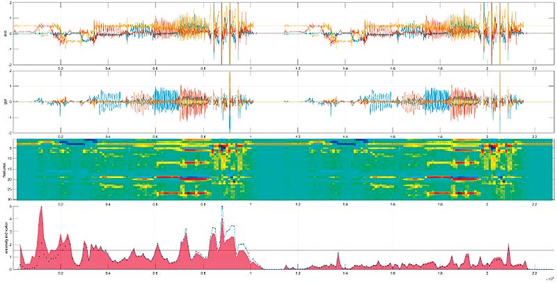
Figure 5: A characteristic curve can be extracted from the raw data of several sensors using various filters, thereby making anomalies visible. (Image source: Knowtion)
Can you explain this using a practical example?
Of course; a typical application would be an intelligent hot water tank connected to a photovoltaic system. I start with sensor deployment planning and specify that several temperature sensors as well as pressure and acceleration sensors are needed.
Now the state has to be assessed: Since I know, for example, that the temperature at the solar collector in these parts will only be between -20°C and +50°C, any data outside this range can be omitted. From a purely physical point of view, the water in the tank cannot rise by 30°C from one minute to the next and, as a result, it is also possible to restrict the dynamic behavior over the time or frequency range. Moreover, a temperature difference of one degree does not have an effect on the system. The data therefore only needs to be analyzed down to an accuracy level of one degree.
The next step is to identify the relevant parameters for the task, e.g. protecting against overheating. In this respect, the temperature of the solar collectors, the cold and hot water inflow, the heat exchanger, and the burner plays a key role. Their data must be filtered out from the sensor fusion. Nothing else needs to be included in the analysis. This is followed by other filters to further reduce the amount of data. This means it is primarily about the parameter identification that influences my overall system.
Selected, filtered data are now available. What is the next step?
Certain patterns and anomalies can now be detected via statistical filters, for instance – and these are the interesting points in order to detect overheating at an early stage in our example. By filtering out the anomalies, I am able to limit their data analysis.
In order to describe the anomalies, extreme system values, i.e. the minimum and maximum values and the turning points, have to be explained mathematically. With cloud and edge analytics this is achieved through differential equations. However, these are too extensive for embedded analytics. We have, therefore, replaced the mathematical curve discussion with a self-learning iteration method. In principle, this is not high-level science, but mathematics taught to the first year students on every basic science course. For the extraction and subsequent visualization of data, a two-dimensional representation is helpful, as it allows you to choose a three-dimensional representation in order to place certain identified parameters in the z-axis of the representation. This is basically comparable to a “topological map” of the sensor data.
How did you proceed with this?
We chose a three-dimensional analysis method in order to make the extreme values recognizable and to subsequently compare the sensor model data. It is already possible to see here that some parameters have very little or no influence on the anomalies. This data can then be neglected or filtered out, as deemed necessary. In order to explain the previously described “topological landscape (figure 5) mathematically, we divided it into less than 100 sub-segments and specified each segment with just 10 measuring points for the iteration, thereby limiting the required storage space from the outset. We defined the difference between the model data and the deviating data as ±1.5%. These are the detection limits of the anomalies.
We then implemented a self-learning iteration method on a STM32 F4 from ST Microelectronics using the so-called dictionary method. This entailed programming iterative queries that determine which mathematical function from the dictionary is to be used to replace which subsection of the sensor function. In just three or four query loops, we arrived at a result that describes the sensor characteristic curve with basic mathematical functions – in other words, an exact modeling of the system that immediately identifies anomalies. The “Sensor Function Dictionary” contains only 5 basic mathematical functions, such as radial basic functions (RBF) or linear functions. The self-learning approach further reduced the segments and the amount of data, meaning just 30 segments were needed, i.e. 300 instead of 400 data points. This was all achieved in real time.
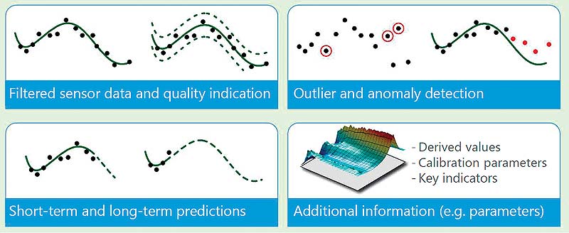
Figure 6: The three-dimensional image of the filtered sensor data enables excellent identification of extreme points. (Image source: Knowtion)
Can this be achieved with any MCU?
In theory yes, in practice no. When processing sensor signals from several sensors (sensor fusion), the real-time capability of the MCU is the main focus of attention. Extremely efficient programming is required for time-synchronous processes, e.g. MEMS sensors with six degrees of freedom. When it comes to time-critical measurements, we discovered that programming on the HAL (high abstraction layer) can lead to measurement errors in the time domain, or that the dynamic changes of the anomalies to be detected were insufficient. The consequence of this was the decision in favor of low-level programming. The memory requirement depends on the previous sensor deployment planning. We chose the STM32, as the analog and digital peripherals combined with the direct response via the low-level allow assembler-based programming in order to implement sensor fusion with the existing RAM and ROM.
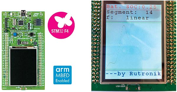
Figure 7: The STM32 has sufficient memory and performance for processing sensor fusion data and enables, for example, predictive maintenance as an embedded real-time system. (Image source: Rutronik)
Is this process now tailored to a specific application?
No, the self-learning algorithms allow us to map any non-linear system of all sensor types and sensor fusions. In addition, it also meets all other requirements placed on embedded analytics: It works offline, i.e. without a cloud, in embedded real-time systems, runs on a standard ARM MCU, and is both robust and scalable.
What was the biggest obstacle during the development phase?
That it demands comprehensive know-how in various disciplines. And this, in turn, requires a whole team of experts. When selecting parameters and pattern matching or determining anomalies, the physical overall system has to be understood fully. It also requires extensive knowledge of all types of sensors and how they work in order to select the appropriate higher mathematics and self-learning algorithms. We have the big advantage of having in-house sensor specialists, analog specialists, and MCU embedded specialists within the project group. In addition, we benefited greatly from the previous research carried out by our partner universities and the specialists in our third party hardware and software specialist network, for example at Knowtion, which specializes in sensor fusion and automatic data analysis.
We can summarize this RUTRONIK proof of concept development as follows: Artificial intelligence and machine learning at the embedded MCU level is not simply a software task. A comprehensive physical and electrochemical understanding of the sensors and how they function with regard to process anomalies is absolutely necessary in order to implement predictive maintenance. The RUTRONIK engineering resources required for this are available to our customers and provide the necessary support for selecting perfectly coordinated products.
Rutronik | www.rutronik.com