


This technical note provides the mathematics code and guidance for engineers implementing a tilt-compensated electronic compass (eCompass).
by Talat Ozyagcilar, Applications Engineer, Freescale Semiconductor
The eCompass uses a three axis accelerometer and three axis magnetometer. The accelerometer measures the components of the earth’s gravity and the magnetometer measures the components of earth’s magnetic field (the geomagnetic field). Since both the accelerometer and magnetometer are fixed on the Printed Circuit Board (PCB), their readings change according to the orientation of the PCB.
If the PCB remains flat, then the compass heading could be computed from the arctangent of the ratio of the two horizontal magnetic field components. Since, in general, the PCB will have an arbitrary orientation, the compass heading is a function of all three accelerometer readings and all three magnetometer readings.
The tilt compensated eCompass algorithm actually calculates all three angles (pitch, roll, and yaw or compass heading) that define the PCB orientation. The eCompass algorithms can therefore also be used to create a 3 D Pointer with the pointing direction defined by the yaw and pitch angles. The accuracy of an eCompass is highly dependent on the calculation and subtraction in software of stray magnetic fields both within, and in the vicinity of, the magnetometer on the PCB. By convention, these fields are divided into those that are fixed (termed Hard Iron effects) and those that are induced by the geomagnetic field (termed Soft Iron effects).
Any zero field offset in the magnetometer is normally included with the PCB’s Hard Iron effects and is calibrated at the same time. This document describes a simple three element model to compensate for Hard Iron effects. This three element model should suffice for many situations. For convenience, the remainder of this document assumes that the eCompass will be implemented within a mobile phone.
Coordinate System and Package Alignment
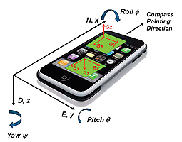
This application note uses the industry standard “NED” (North, East, Down) coordinate system to label axes on the mobile phone. The x axis of the phone is the eCompass pointing direction; the y axis points to the right and the z axis points downward (see Figure 1).
A positive Yaw angle ψ is defined to be a clockwise rotation about the positive z axis. Similarly, a positive pitch angle θ and positive roll angle φ are defined as clockwise rotations about the positive y and positive x axes respectively.
It is crucial that the accelerometer and magnetometer outputs are aligned with the phone coordinate system. Different PCB layouts may have different orientations of the accelerometer and magnetometer packages and even the same PCB may be mounted in different orientations within the final product.
For example, in Figure 1, the accelerometer y- axis output Gy, is correctly aligned, but the x-axis Gx and z-axis Gz signals are inverted in sign. Also in Figure 1, the magnetometer output Bz is correct, but the y-axis signal should be set to Bx and the x-axis signal should be set to -By.
Once the package rotations and reflections are applied in software, a final check should be made while watching the raw accelerometer and magnetometer data from the PCB:
1. Place the PCB flat on the table. The z-axis accelerometer should read +1g and the x and y axes negligible values. Invert the PCB so that the z axis points upwards and verify that the z- axis accelerometer now indicates -1g. Repeat with the y-axis pointing downwards and then upwards to check that the y axis reports 1g and then reports -1g. Repeat once more with the x- axis pointing downwards and then upwards to check that the x-axis reports 1g and then -1g.
2. The horizontal component of the geomagnetic field always points to the magnetic north pole. In the northern hemisphere, the vertical component also points downward with the precise angle, being dependent on location. When the PCB x-axis is pointed northward and downward, it should be possible to find a maximum value of the measured x component of the magnetic field. It should also be possible to find a minimum value when the PCB is aligned in the reverse direction. Repeat the measurements with the PCB y- and z-axes aligned first with, and then against, the geomagnetic field which should result in maximum and minimum readings in the y- and then z-axes.
Accelerometer and Magnetometer Outputs as a Function of Phone Orientation
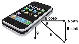
Any orientation of the phone can be modeled as resulting from rotations in yaw, pitch and the roll applied to a starting position with the phone flat
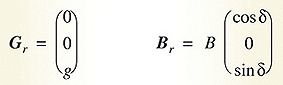
and pointing northwards. The accelerometer, Gr, and magnetometer, Br, readings in this starting reference position are (see Figure 2).
The acceleration due to gravity is g = 9.81 ms-².
B is the geomagnetic field strength which varies over the earth’s surface from a minimum of 22μT over South America to a maximum of 67μT south of Australia. δ is the angle of inclination of the geomagnetic field measured downwards from horizontal and varies over the earth’s surface from -90° at the south magnetic pole, through zero near the equator to +90° at the north magnetic pole. Detailed geomagnetic field maps are available from the World Data Center for Geomagnetism at http://wdc.kugi.kyoto-u.ac.jp/igrf/
There is no requirement to know the details of the geomagnetic field strength nor inclination angle in order for the eCompass software to function. The magnetic field strength B and the inclination angle δ, cancel in the angle calculations (see Equations 20, 21 and 22).
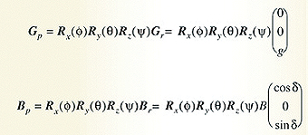
The phone accelerometer, Gp, and magnetometer, Bp, readings measured after the three rotations Rz(ψ) then Ry(θ) and finally Rx(φ) are described by the equations:
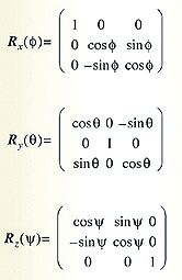
The three rotation matrices referred to in Equations 3 and 4 are:
Equation 3 assumes that the phone is not undergoing any linear acceleration and that the accelerometer signal Gp is a function of gravity and the phone orientation only. A tilt-compensated eCompass will give erroneous readings if it is subjected to any linear acceleration.
Equation 4 ignores any stray magnetic fields from Hard and Soft Iron effects. The standard way of modeling the Hard Iron effect is as an additive magnetic vector, V, which rotates with the phone PCB and is therefore independent of phone orientation. Since any magnetometer sensor zero flux offset is also independent of phone orientation,
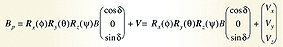
it simply adds to the PCB Hard Iron component and is calibrated and removed at the same time.
Equation 4 then becomes:
where Vx, Vy, and Vz, are the components of the Hard Iron vector. Equation 8 does not model Soft Iron effects.
Tilt-Compensation Algorithm
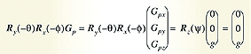
The tilt-compensated eCompass algorithm first calculates the roll and pitch angles φ and θ from the accelerometer reading by pre-multiplying Equation 3 by the inverse roll and pitch rotation matrices giving:
where the vector contains the three components of gravity measured by the accelerometer.
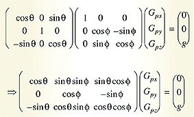
Expanding Equation 9 gives:
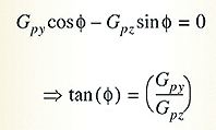
The y component of Equation 11 defines the roll angle φ as:
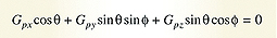
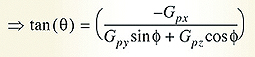
(Eqn. 12) The x component of Equation 11 gives the pitch angle θ as:
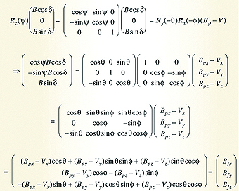
With the angles φ and θ known from the accelerometer, the magnetometer reading can be de-rotated to correct for the phone orientation using Equation 5:
The vector represent the components of the magnetometer sensor after correcting for the Hard Iron offset and after de-rotating to the flat plane where θ = φ = 0.
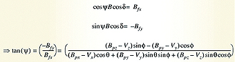
The x and y components of Equation 19 give:
Equation 22 allows a solution for the yaw angle ψ where ψ is computed relative to magnetic north. The yaw angle ψ is therefore the required tilt-compensated eCompass
heading.
Since Equations 13, 15 and 22 have an infinite number of solutions at multiples of 360°, it is standard convention to restrict the solutions for roll, pitch and yaw to the range -180° to 180°.
A further constraint is imposed on the pitch angle to limit it to the range -90° to 90°. This ensures only one unique solution exists for the compass, pitch and roll angles for any phone orientation. Equations 13 and 22 are therefore computed with a software ATAN2 function (with output angle range -180° to 180°) and Equation 15 is computed with a software ATAN function (with output angle range -90° to 90°).
Estimation of the Hard Iron Offset V
Equation 22 assumes knowledge of the Hard Iron offset V, which is a fixed magnetic offset adding to the true magnetometer sensor output. The Hard Iron offset is the sum of any intrinsic zero field offset within the magnetometer sensor itself plus permanent magnetic fields within the PCB generated by magnetized ferromagnetic materials. It is quite normal for the Hard Iron offset to greatly exceed the geomagnetic field. Therefore, an accurate Hard Iron estimation and subtraction are required to avoid Equation 22 jamming and returning compass angles within a limited range only. It is common practice for magnetometer sensors to be supplied without zero field offset calibration since the standard Hard Iron estimation algorithms will compute the sum of both the magnetometer sensor zero field offset and the PCB Hard Iron offset.
In the absence of any Hard Iron effects, the locus of the magnetometer output under arbitrary phone orientation changes lies on the surface of a sphere in the space of Bpx, Bpy and Bpz with a radius equal to the magnitude of the geomagnetic field B. In the presence of Hard Iron effects, the locus of the magnetic measurements is simply displaced by the Hard Iron vector V so that the origin of the sphere is equal to the Hard Iron offset Vx, Vy and Vz. The Hard Iron Offset can then be simply computed by
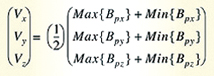
monitoring the minimum and maximum values of the x, y, and z components of the magnetometer readings and estimating the Hard Iron offset components by:
The minimum and maximum magnetometer readings can either i) be measured and the Hard Iron offset computed and stored at factory calibration time or ii) be tracked on the fly using the random orientations of the phone to continuously self-calibrate the phone.
SOFTWARE IMPLEMENTATION
The reference C# code uses integer operands only and makes no calls to any external mathematical libraries. Custom functions are provided in this document for all the trigonometric and numerical calculations required. It is provided in the Application Note AN4248 from Freescale Semiconductor and can be found at www.element14.com/freescale